Predator-prey equations
The predator-prey equations is an ecological system of two linked equations that models two species that depend on each other: One is the prey, which provides food for the other, the predator. Both prey and predator populations grow if conditions are right. Alfred J. Lotka found these equations in 1925.[1] Vito Volterra found them, independently, in 1926. For this reason, the equations are also called Lotka-Volterra equations.[2]
The equations themselves are non-linear differential equations.
Pre-conditions
There are a number of pre-conditions
- The prey population always finds food
- The size of the predator population only depends on the size of the prey population
- The rate of change of a population depends on its size
- There are no changes in the environment which would favor one species. Genetic changes are not important
- Predators have limitless appetite
In this case the solution of the differential equations is deterministic and continuous. This means that the generations of both the predator and prey are overlapping all the time.[3]
Lotka-Volterra rules
The solutions to the equations lead to the Lotka-Volterra rules:
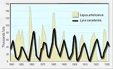
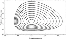
- There are periodic changes is the populations of predator and prey. The changes in the population of predators follow that of the prey.
- Looking at longer periods of time: the average number of predators, and prey is constant so long as the environment is stable.
- If the number of predators is reduced, the number of prey animals increase.
A general predator-prey Model
Consider two populations whose sizes at a reference time t are denoted by x(t), y(t), respectively. The functions x and y might might denote population numbers or concentration (number per area) or some other scaled measure of the population sizes, but are taken to be continuous functions. Changes in population size with time are describing by the time derivatives and , respectively.[4]


Kolmogorov equations
Kolmogorov's predator-prey model refers to the general model describing dynamics of interacting populations in terms of two autonomous differential equations:[4]


where and denote the respective per capita growth rates of the two species satisfying and . This general model is often called Kolmogorov's predator-prey model.[5][6]


Applications
In one of his books, Volterra provided statistics on the number of certain cartilagenous fish caught at some Italian ports in the Mediterranean.[7] Volterra used the term "sélaciens", which refers to sharks. These often prey on other fish. In the table, Volterra provided numbers for 1905, and 1910 to 1923:
| 1905 | 1910 | 1911 | 1912 | 1913 | 1914 | 1915 | 1916 | 1917 | 1918 | 1919 | 1920 | 1921 | 1922 | 1923 | |
| Trieste | – | 5,7 | 8,8 | 9,5 | 15,7 | 14,6 | 7,6 | 16,2 | 15,4 | – | 19,9 | 15,8 | 13,3 | 10,7 | 10,2 |
| Fiume[8] | – | – | – | – | - | 11,9 | 21,4 | 22,1 | 21,2 | 36,4 | 27,3 | 16 | 15,9 | 14,8 | 10,7 |
| Venice | 21,8 | – | – | – | - | – | – | - | – | – | 30,9 | 25,3 | 25,9 | 26,8 | 26,6 |
He observed that between 1915 and 1920, more of these fish were caught. He expained this as follows: During the First World War, less fishing was done. For this reason, there were more prey animals, so the number of predators increased. After the war, fishing increased again, reducing the number of prey animals. This also led to a decrease in the number of predators, which can be seen in the table above.
The use of the first Lotka-Volerra rule in economics is known as pork cycle.
Extensions
The predator-prey equations have also been the foundation of other work. Volterra himselft extended it to be able to model intraspecific competition. Intraspecific competition occurs when two aninimals of the same species compete for limited resources. Intraspecific competition is an important factor to regulate population density. It is also important to be able to adapt to a changing environment (and for evoution). Volterra did this by adding new terns to the equation.
Most of Volerra's work is about extending the model to be able to handle more than two classes of animals interacting.
Related pages
References
- Lotka A.J. 1925. Elements of physical biology. Williams and Wilkins.
- Leigh E.R. 1968. The ecological role of Volterra's equations, in Some Mathematical Problems in Biology. A modern discussion using Hudson's Bay Company data on lynx and hares in Canada from 1847 to 1903.
- Cooke, D.; Hiorns, R. W.; et al. (1981). The Mathematical Theory of the Dynamics of Biological Populations. Vol. II. Academic Press.
- Caraballo, Tomás; Colucci, Renato; Han, Xiaoying (August 2016). "Semi-Kolmogorov models for predation with indirect effects in random environments". Discrete and Continuous Dynamical Systems - Series B. 21 (7): 2129–2143. doi:10.3934/dcdsb.2016040. ISSN 1531-3492. S2CID 125795329.
- "Deterministic mathematical models in population ecology. By H.I.Freedman, The University of Alberta. Pure and Applied Mathematics: A series of monographs and textbooks, volume 57. Marcel Dekker, Inc., New York, 1980. x + 254 pp. US. $29.75. ISBN 0-8247-6653-9". Canadian Journal of Statistics. 10 (4): 315. 1982. doi:10.2307/3556198. JSTOR 3556198.
- Mathematical Models in Population Biology and Epidemiology. Texts in Applied Mathematics. Vol. 40. 2012. doi:10.1007/978-1-4614-1686-9. ISBN 978-1-4614-1685-2.
- Volterra, Vito (1931). Leçons sur la Théorie Mathématique de la Lutte pour la Vie., 1931. Gauthier-Villars.
- Fiume is called Rijeka today. From 1805 to 1945 it was part of Italy. At the end of World War II, about 80% of its inhabitants were Italians.
Further reading
- "The Predator-Prey Equations" (PDF).
- "Models of Preditor-Prey Relationships" (PDF). Tyler Blaszak.
- "Lynx vs Hare Cycle (from Northwest Territories)" (PDF).
Other websites
- "Lynx-Snowshoe Hare Cycle". Environment and Natural Resources (Canada). The most commonly cited example of these equations
- "Predatory-Prey Relationships: The Fox and the Rabbit game". Jackie Sibenaller. MnSTEP Teaching Activity Collection.