

/en/excel2010/cell-basics/content/
When you open a new blank workbook, the cells are set to a default size. You have the ability to modify cells, as well as to insert and delete columns, rows, and cells as needed. In this lesson, you will learn how to change row height and column width, insert and delete rows and columns, wrap text in a cell, and merge cells.
By default, every row and column of a new workbook is set to the same height and width. Excel allows you to modify column width and row height in different ways.
 becomes a double arrow
  .
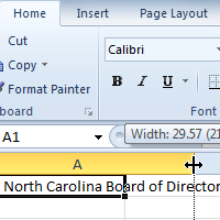
. Positioning mouse over the column line
 Increasing the column width
 Increased column width
If you see pound signs (#######) in a cell, it means the column is not wide enough to display the cell content. Simply increase the column width to show the cell content.
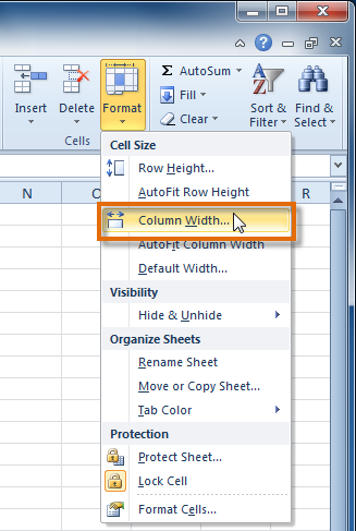 Increasing the column width
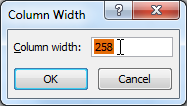 Increasing column width to 258 pixels
Select AutoFit Column Width from the format drop-down menu, and Excel will automatically adjust each selected column so all of the text will fit.
 becomes a double arrow
  .
.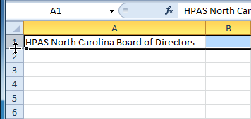 Positioning the mouse over the row line
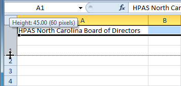 Increasing the row height
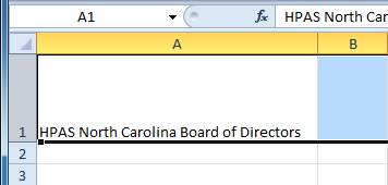 Increased row height
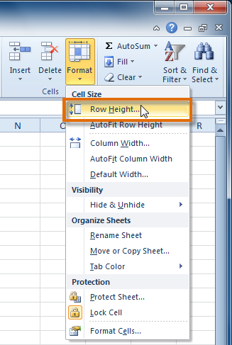 Increasing the column width
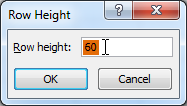 Increasing row height to 60 pixels
Select AutoFit Row Height from the format drop-down menu, and Excel will automatically adjust each selected row so all of the text will fit.
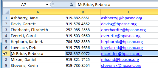 Selecting the row
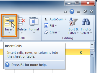 Selecting the Insert Cells command
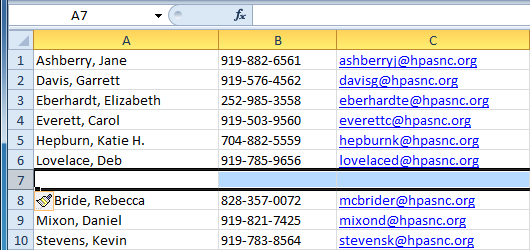 The inserted row
When inserting new rows, columns, or cells, you will see the Insert Options button  by the inserted cells. This button allows you to choose how Excel formats them. By default, Excel formats inserted rows with the same formatting as the cells in the row above them. To access more options, hover your mouse over the Insert Options button and click the drop-down arrow that appears.
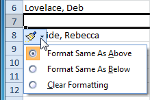 Accessing Insert Options
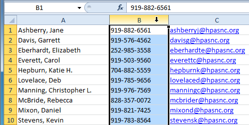 Selecting the column
 Selecting the Insert Cells command
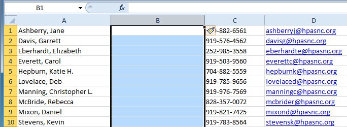 The inserted column
By default, Excel formats inserted columns with the same formatting as the column to the left of them. To access more options, hover your mouse over the Insert Options button and click the drop-down arrow that appears.
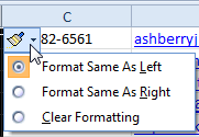 Accessing Insert Options
When inserting rows and columns, make sure to select the row or column by clicking its heading so all of the cells in that row or column are selected. If you select just a cell in the row or column, only a new cell will be inserted.
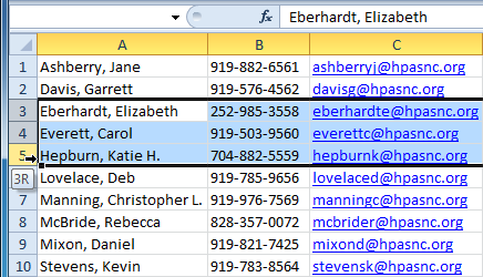 Selecting the rows
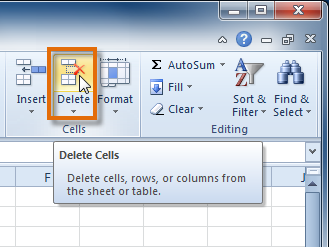 Selecting the Delete command
 The rows are deleted
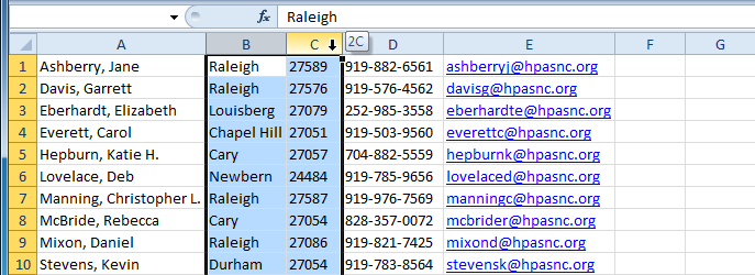 Selecting the columns
 Selecting the Delete command
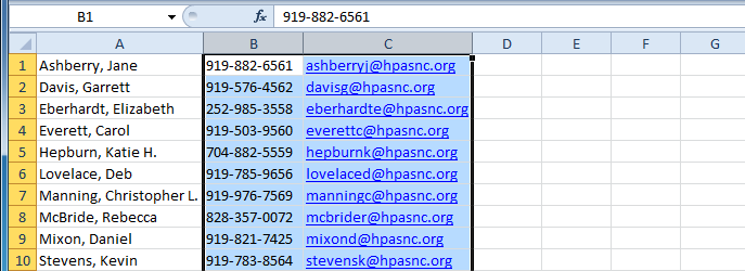 The columns are deleted
If a cell contains more text than can be displayed, you can choose to wrap the text within the cell or merge the cell with empty adjoining cells. Wrap text to make it display on multiple lines of the cell. Merge cells to combine adjoining cells into one larger cell.
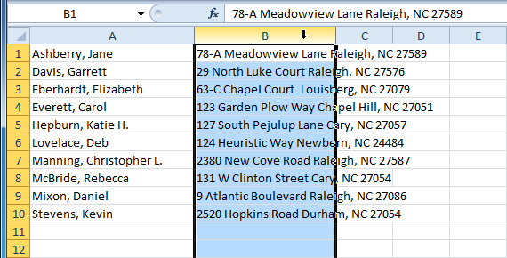 Selecting cells
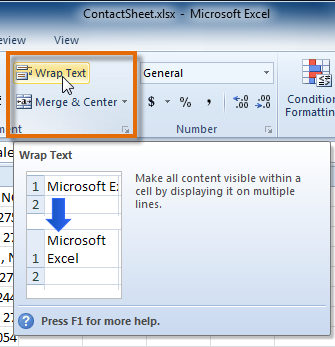 Selecting the Wrap Text command
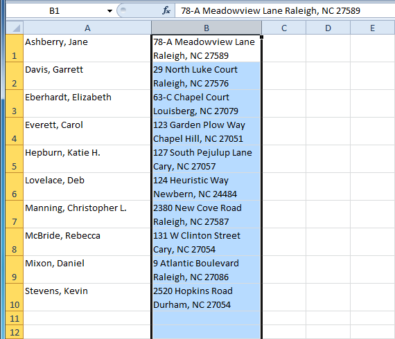 Cells with wrapped text
If you change your mind, reclick the Wrap Text command to unwrap the text.
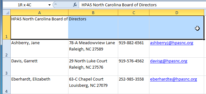 Selecting A1:D1 (A1, B1, C1, D1)
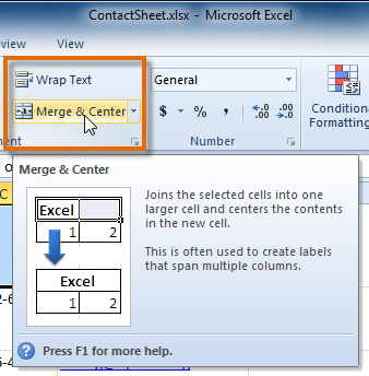 Selecting the Merge & Center command
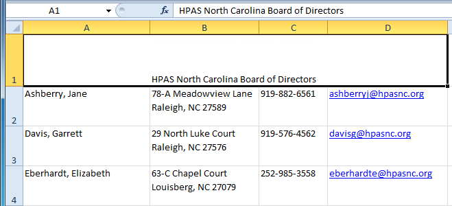 A1 after merging with B1:D1
If you change your mind, reclick the Merge & Center command to unmerge the cells.
Click the drop-down arrow next to the Merge & Center command on the Home tab. The merge drop-down menu appears.
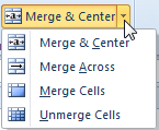 Accessing more Merge options
Although merging cells can be useful, it can also cause problems with some spreadsheets. Watch the video below to learn about some of the problems with merging cells.
/en/excel2010/formatting-cells/content/