Lesson 15: Working with Functions

/en/googlespreadsheets/types-of-cell-references/content/

Introduction

A function is a predefined formula that performs calculations using specific values in a particular order. Excel includes many common functions that can be used to quickly find the sum, average, count, maximum value, and minimum value for a range of cells. In order to use functions correctly, you'll need to understand the different parts of a function and how to create arguments to calculate values and cell references.

Watch the video below to learn how to create functions.

The parts of a function

Similar to entering a formula, the order in which you enter a function into a cell is important. Each function has a specific order—called syntax—that must be followed in order for the function to calculate properly. The basic syntax to create a formula with a function is to insert an equals sign (=), a function name (AVERAGE, for example, is the function name for finding an average), and an argument. Arguments contain the information you want the formula to calculate, such as a range of cell references.
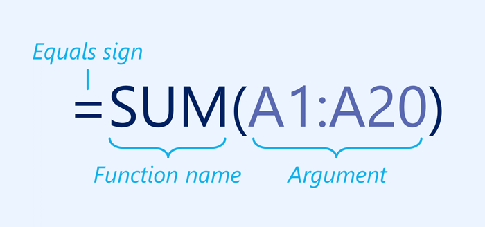
Syntax of a basic function

Working with arguments

Arguments can refer to both individual cells and cell ranges and must be enclosed within parentheses. You can include one argument or multiple arguments, depending on the syntax required for the function.

For example, the function =AVERAGE(B1:B9) would calculate the average of the values in the cell range B1:B9. This function contains only one argument.
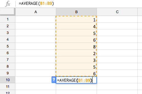
A function containing one argument

Multiple arguments must be separated by a comma. For example, the function =SUM(A1:A3, C1:C2, E1) will add the values of all of the cells in the three arguments.
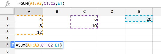
A function containing multiple arguments

Creating a function

Google Sheets has a variety of functions available. Here are some of the most common functions you'll use:

  • SUM: This function adds all of the values of the cells in the argument.
  • AVERAGE: This function determines the average of the values included in the argument. It calculates the sum of the cells and then divides that value by the number of cells in the argument.
  • COUNT: This function counts the number of cells with numerical data in the argument. This function is useful for quickly counting items in a cell range.
  • MAX: This function determines the highest cell value included in the argument.
  • MIN: This function determines the lowest cell value included in the argument.

To create a function using the Functions button:

The Functions button allows you to automatically return the results for a range of cells. The answer will display in the cell below the range.
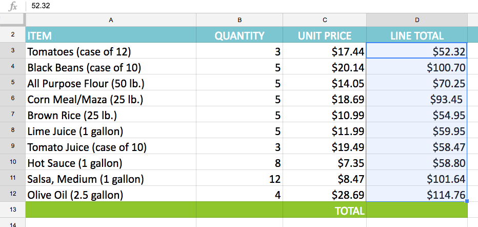
  1. Select the range of cells you want to include in the argument. In our example, we'll select D3:D12.Selecting a range of cells


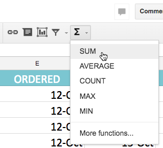
  2. Click the Functions button, then select the desired function from the drop-down menu. In our example, we'll select SUM.
    Selecting SUM
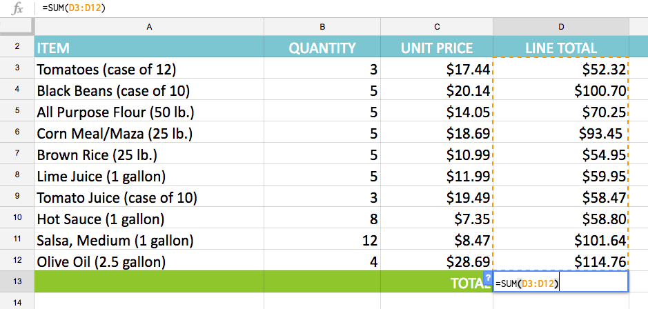
  3. In the cell directly below the selected cells, the function appears.
    The function in the adjacent cell
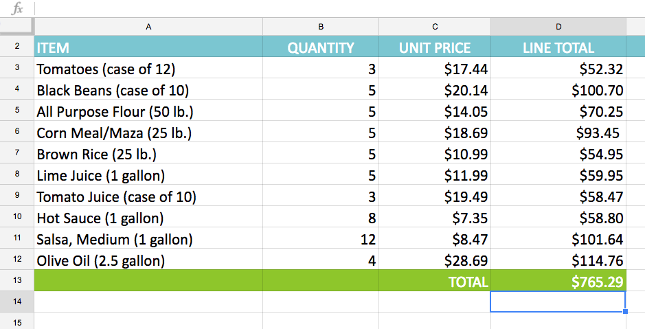
  4. Press the Enter key on your keyboard. The function will be calculated, and the result will appear in the cell. In our example, the sum of D3:D12 is $765.29.
    The result

To create a function manually:

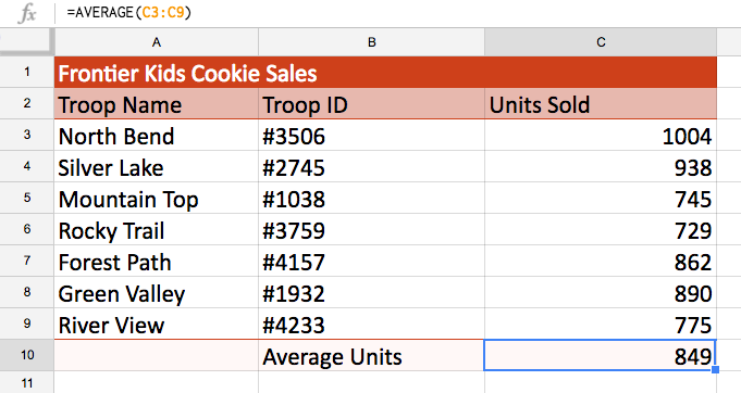
If you already know the function name, you can easily type it yourself. In the example below, which is a tally of cookie sales, we'll use the AVERAGE function to calculate the average number of units sold by each troop.
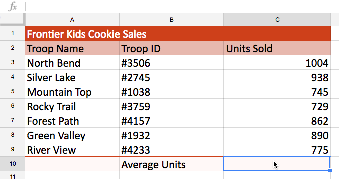
  1. Select the cell where the answer will appear. In our example, we'll select C10.
    Selecting a range of cells
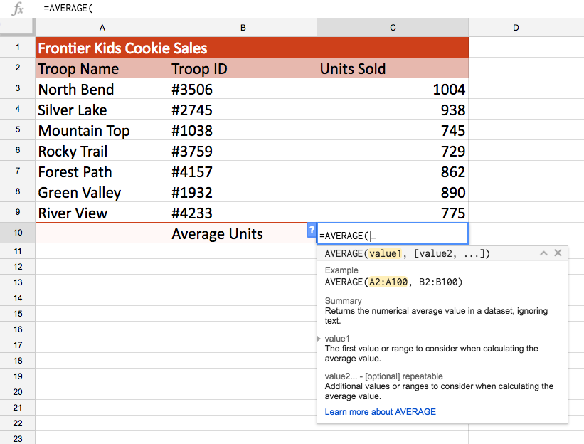
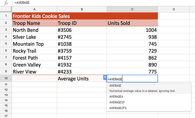
  2. Type the equals sign (=), then type the desired function name. You can also select the desired function from the list of suggested functions that appears below the cell as you type. In our example, we'll type =AVERAGE.
    Typing the function =AVERAGE
  3. When typing a function manually, Google Sheets also displays a window that lists the specific arguments the function needs. This window appears when the first parenthesis is typed and stays visible as the arguments are typed.
    Google Sheets argument window
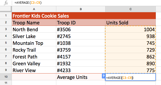
  4. Enter the cell range for the argument inside parentheses. In our example, we'll type (C3:C9). This formula will add the values of cells C3:C9, then divide that value by the total number of values in the range.Entering the cell range
  5. Press the Enter key on your keyboard, and the answer appears.
    Displaying the result

Google Sheets will not always tell you if your function contains an error, so it's up to you to check all of your functions. To learn how to do this, read our article on why you should Double-Check Your Formulas.

Google Sheets function list

If you have experience using spreadsheets and want to use Google Sheets to make more advanced calculations, you can explore the Google Sheets function list. It is a handy reference for hundreds of financial, statistical, and data analysis functions.
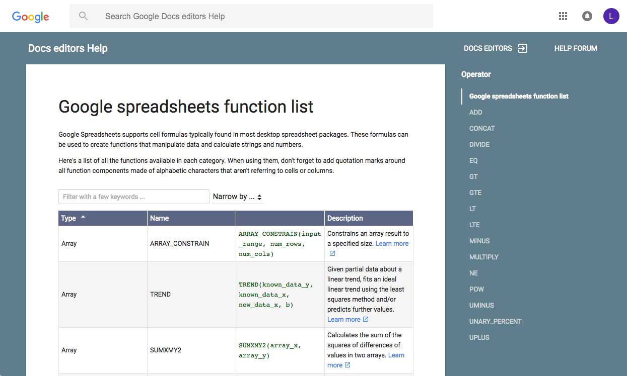
The Google Spreadsheets function list

To access the function list:

Click the Functions button and select More functions... from the drop-down menu. The Google sheets function list will appear in a new browser tab.
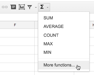
Selecting More functions

If you're comfortable with basic functions, you may want to try a more advanced one like VLOOKUP. You can check out our article on How to Use Excel's VLOOKUP Function for more information. Like most functions, VLOOKUP works the same way in Excel and Google Sheets.
Challenge!

  1. Open our example file. Make sure you're signed in to Google, then click File > Make a copy.
  2. Select the Challenge sheet.
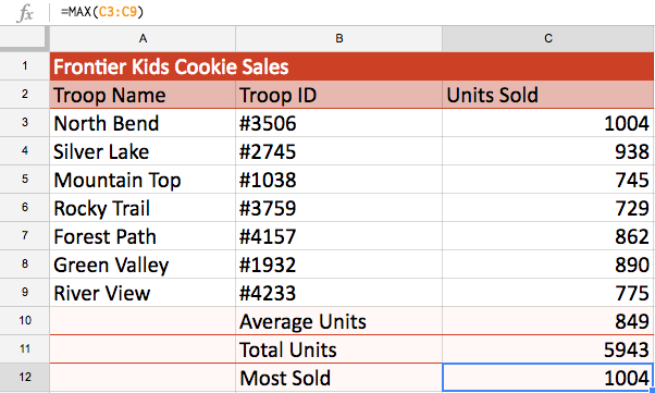
  3. Fix the formula in cell C10 so it finds the average number of units sold by all of the troops.
  4. In cell C11, write a function that will find the total amount of units sold by all of the troops.
  5. In cell C12, write a function that will find the largest number of units sold by a troop.
  6. When you're finished, your spreadsheet should look something like this:
    functions challenge example

/en/googlespreadsheets/sorting-and-filtering-data/content/