This article was co-authored by wikiHow Staff. Our trained team of editors and researchers validate articles for accuracy and comprehensiveness. wikiHow's Content Management Team carefully monitors the work from our editorial staff to ensure that each article is backed by trusted research and meets our high quality standards.
The wikiHow Tech Team also followed the article's instructions and verified that they work.
This article has been viewed 572,778 times.
Learn more...
This wikiHow teaches you how to create and insert a new column to a pivot table in Microsoft Excel with the pivot table tools. You can change an existing row, field or value to a column, or create a new calculated field column with a custom formula.
Steps
Changing a Field to Column
-
1Open the Excel file with the pivot table you want to edit. Find and double-click your Excel file on your computer to open it.
- If you haven't made your pivot table yet, open a new Excel document and create a pivot table before continuing.
-
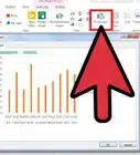
2Click any cell on the pivot table. This will select the table, and show the pivot table Analyze and Design tabs on the toolbar ribbon at the top.Advertisement
-
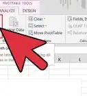
3Click the Pivot Table Analyze tab at the top. You can find this tab alongside other tabs like Formulas, Insert, and View at the top of the app window. It will show your pivot table tools on the toolbar ribbon.
- On some versions, this tab may just be named Analyze, and on others, you can find it as Options under the "Pivot Table Tools" heading.
-
4Click the Field List button on the toolbar ribbon. You can find this button on the right-hand side of the pivot table Analyze tab. It will open a list of all the fields, rows, columns, and values in the selected table.
-
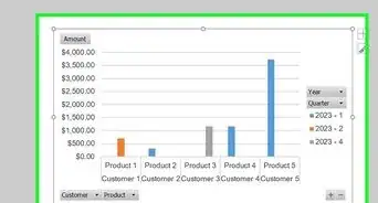
5Check the box next to any item on the FIELD NAME list. This will calculate the summary of your original data in the selected category, and add it to your pivot table as a new column.
- Typically, non-numeric fields are added as rows, and numeric fields are added as columns by default.
- You can uncheck the checkbox here anytime to remove the column.
-
6Drag and drop any field, row or value item to the "Columns" section. This will automatically move the selected category to the Columns list, and re-design your pivot table with the newly added column.


Adding a Calculated Field
-
1Open the Excel document you want to edit. Double-click the Excel document that contains your pivot table.
- If you haven't yet made the pivot table, open a new Excel document and create a pivot table before continuing.
-
2Select the pivot table you want to edit. Click the Pivot Table on your worksheet to select and edit it.
-
3Click the Pivot Table Analyze tab. This tab is in the middle of the toolbar ribbon at the top of the Excel window. It will open your pivot table tools on the toolbar ribbon.
- On different versions, this tab may be named Analyze, or Options under the "Pivot Table Tools" heading.
-
4Click the Fields, Items, & Sets button on the toolbar ribbon. This button looks like an "fx" sign on a table icon on the far-right end of the toolbar. It will open a drop-down menu.
-
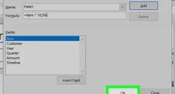
5Click Calculated Field on the drop-down menu. It will open a new window where you can add a new, custom column to your Pivot Table.
-
6Enter a name for your column in the "Name" field . Click the Name field, and type in the name you want to use for your new column. This name will appear at the top of the column.
-
7Enter a formula for your new column in the "Formula" field. Click the Formula field below Name, and type the formula you want to use for calculating your new column's data values.
- Make sure you type the formula on the right side of the "=" sign.
- Optionally, you can also select an existing column, and add it to your formula as a value. Select the field you want to add in the Fields section here, and click Insert Field to add it to your formula.
-
8Click OK. Doing so will add the column to the right side of your pivot table.


Warnings
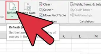
- Always remember to save your work when you're done.⧼thumbs_response⧽


About This Article

1. Click on the PivotTable.
2. Click the checkbox of the field you want to add.
3. Right-click on the added field.
4. Select Move to... Column Labels or Values.