wikiHow is a “wiki,” similar to Wikipedia, which means that many of our articles are co-written by multiple authors. To create this article, 20 people, some anonymous, worked to edit and improve it over time.
This article has been viewed 538,011 times.
Learn more...
Have you inherited a document with the dates in the wrong format? Maybe you were the one who made the mistake, or you simply have decided to go a different route. Whatever the reason, you can quickly and easily change the date format in Microsoft Excel. You can choose to change the date format for a specific set of data within an Excel sheet, or you can change the standard date format for your entire computer in order to apply that format to all future Excel sheets.
Steps
Changing the Standard Date Format
-
1Navigate to the time and date settings. In order to change the standard date format for any new Excel sheet, you will need to change the overarching date format for you computer. First, click the Start button. The next step will depend on which operating system you are using:[1]
- If you are using Windows Vista or Windows 8: Open the Control Panel. Then, click "Clock, Language, and Region." Alternately, in Windows 8, open the Settings folder and select "Time & language".
- If you are using Windows XP: Open the Control Panel. Then, click "Date, Time, Language, and Regional Options."
-
2Navigate to the Regional options. Again, the navigational steps vary from operating system to operating system.
- If you are using Windows 8: In the Clock, Language, and Region folder, select "Change date, time, or number formats" from beneath the "Region" heading.
- If you are using Windows Vista: Open the Regional and Language Options dialog box. Then, select the Formats tab.
- If you are using Windows XP: Open the Regional and Language Options dialog box. Then, select the Regional Options tab.
Advertisement -
3Prepare to customize the format. If you are using Windows 8: Make sure that the Formats tab is open. If you are using Windows Vista: Click Customize this format. If you are using Windows XP: Click Customize.[2]
-
4Choose a date format. You will have options for the short date and the long date. The short date refers to the abbreviated version: e.g. 6/12/2015. The long date refers to the wordier form: e.g. December 31, 1999. The formats that you select here will be standardized across all Windows applications, including Excel. Click "OK" to apply your choices.
- Review the short date options. June 2, 2015 is used as an example.
- M/d/yyyy: 6/2/2015
- M/d/yy: 6/2/15
- MM/dd/yy: 06/02/15
- MM/dd/yyyy: 06/02/2015
- yy/MM/dd: 15/06/02
- yyyy-MM-dd: 2015-06-02
- dd-MMM-yy: 02-Jun-15
- Review the long date options. June 2, 2015 is used as an example.
- dddd, MMMM dd, yyyy: Friday, June 02, 2015
- dddd, MMMM d, yyyy: Friday, June 2, 2015
- MMMM d, yyyy: June 2, 2015
- dddd, d MMMM, yyyy: Friday, 2 June, 2015
- d MMMM, yyyy: 2 June, 2015
- Review the short date options. June 2, 2015 is used as an example.


Changing Date Formats for Specific Sets
-
1Open the spreadsheet and highlight all the relevant date fields. If you only want to change the date format for one cell: simply click on that cell.[3]
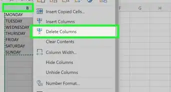
- If the dates are aligned in a column: select and format the entire column by left-clicking on the letter at the top of the column. Then, right-click to bring up an action menu.
- If the dates are laid out in a row: highlight the section or cell that you want to change. Then, left-click on the number at the far-left of the row to select all of the cells.
-
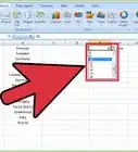
2Select the drop-down "Format" menu from the toolbar. Find the drop-down menu in the "Cells" compartment (between "Styles" and "Editing") while you are in the "Home" tab.
- Alternately: right-click on the number on the far-left of a row or the letter at the top of a given column. This will select all of the cells in that row or column, and it will bring up an action menu. Select "Format Cells" from that menu to format the date for all of the cells in that column.[4]
-
3Select "Format Cells" from the drop-down menu. Look for this option at the bottom of the menu.
-
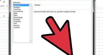
4Navigate to the "Number" tab. Find this on the tab on the far-top-left of the "Format Cells" window, next to "Alignment," "Font," "Border," "Fill," and "Protection." "Number" is usually the default.
-
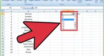
5Select "Date" from the "Category" column at the left of the screen. This will allow you to manually reformat format the date settings.
-
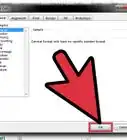
6Select the date format you'd like. Highlight that choice, and click "OK" to save the format. Then, save the file to ensure that your formatting is preserved


Community Q&A
-
QuestionHow do I fix a date error in my spreadsheet?
 Community AnswerIf you're getting the ## sign, that means the column is too small. Go to the top of that column and when your mouse turns to a cross, click and drag to the right. Otherwise, stay on the cell you want to fix, click on format on the menu bar and look for date format.
 -
QuestionI want to add the past month and year to one cell, but 2016 keeps coming back. What can I do?
 Community AnswerYou can concatenate the 2 items. =Month(a1)&"/"&Year(a1) will give "1/2016" as a text field.


References
- ↑ https://support.office.com/en-us/article/Change-the-date-system-format-or-two-digit-year-interpretation-aaa2159b-4ae8-4651-8bce-d4707bc9fb9f#bmchange_the_default_date_format_to_dis
- ↑ http://excelribbon.tips.net/T011575_Setting_a_Default_Date_Format.html
- ↑ https://www.ablebits.com/office-addins-blog/2015/03/11/change-date-format-excel/
- ↑ http://www.extendoffice.com/documents/excel/585-excel-change-american-date-format.html
- ↑ https://support.office.com/en-us/article/Format-a-date-the-way-you-want-8e10019e-d5d8-47a1-ba95-db95123d273e