How to Round in Excel

Last Updated: August 17, 2022 Tested

Using the Increase and Decrease Decimal Buttons

|

Using the ROUND Formula

|

Using Cell Formatting

This wikiHow teaches you how to round the value of a cell using the ROUND formula, and how to use cell formatting to display cell values as rounded numbers.

Method 1

Method 1 of 3:

Using the Increase and Decrease Decimal Buttons

1
Enter the data into your spreadsheet.
2
Highlight any cell(s) you want rounded. To highlight multiple cells, click the top left-most cell of the data, then drag your cursor down and to the right until all cells are highlighted.

Advertisement
3
Click the Decrease Decimal button to show fewer decimal places. It's the button that says .00 → .0 on the Home tab on the “Number” panel (the last button on that panel).
- Example: Clicking the Decrease Decimal button would change $4.36 to $4.4.
4
Click the Increase Decimal button to show more decimal places. This gives a more precise value (rather than rounding). It's the button that says ←.0 .00 (also on the “Number” panel).
- Example: Clicking the Increase Decimal button might change $2.83 to $2.834.

Method 2

Method 2 of 3:

Using the ROUND Formula

1
Enter the data into your spreadsheet.
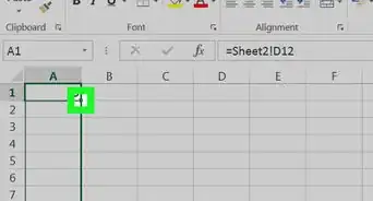
2
Click a cell next to the one you want to round. This allows you to enter a formula into the cell.
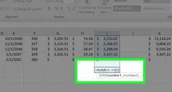
3
Type “ROUND” into the “fx” field. The field is at the top of the spreadsheet. Type an equal sign followed by “ROUND” like this: =ROUND.
4
Type an open parenthesis after “ROUND.” The content of the “fx” box should now look like this: =ROUND(.
5
Click the cell that you want to round. This inserts the cell's location (e.g., A1) into the formula. If you clicked A1, the “fx” box should now look like this: =ROUND(A1.
6
Type a comma followed by the number of digits to round to. For example, if you wanted to round the value of A1 to 2 decimal places, your formula would so far look like this: =ROUND(A1,2.
- Use 0 as the decimal place to round to the nearest whole number.
- Use a negative number to round by multiples of 10. For example, =ROUND(A1,-1will round the number to the next multiple of 10.
7
Type a closed parenthesis to finish the formula. The final formula should look like this (using the example of rounding A1 2 decimal places: =ROUND(A1,2).
8
Press ↵ Enter or ⏎ Return. This runs the ROUND formula and displays the rounded value in the selected cell.
- You can replace ROUND with ROUNDUP or ROUNDDOWN if you know you want to round up or round down to a certain number of decimal points.^{[1]
  X
  Research source}
- Similarly, the formula MROUND will round to the nearest multiple of any specified number.^{[2]
  X
  Research source}

Method 3

Method 3 of 3:

Using Cell Formatting

1
Enter your data series into your Excel spreadsheet.
2
Highlight any cell(s) you want rounded. To highlight multiple cells, click the top left-most cell of the data, then drag your cursor down and to the right until all cells are highlighted.
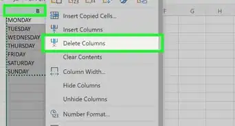
3
Right-click any highlighted cell. A menu will appear.
4
Click Number Format or Format Cells. The name of this option varies by version.
5
Click the Number tab. It's either on the top or side of the window that popped up.
6
Click Number from the category list. It's on the side of the window.
7
Select the number of decimal places you want to round to. Click the down-arrow next to the “Decimal places” menu to display the list of numbers, then click the one you want to select.
- Example: To round 16.47334 to 1 decimal place, select 1 from the menu. This would cause the value to be rounded to 16.5.
- Example: To round the number 846.19 to a whole number, select 0 from the menu. This would cause the value to be rounded to 846.
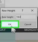
8
Click OK. It's at the bottom of the window. The selected cells are now rounded to the selected decimal place.
- To apply this setting to all values on the sheet (including those you add in the future), click anywhere on the sheet to remove the highlighting, and then click the Home tab at the top of Excel, click the drop-down menu on the “Number” panel, then select More Number Formats. Set the desired “Decimal places” value, then click OK to make it the default for the file.
- In some versions of Excel, you'll have to click the Format menu, then Cells, followed by the Number tab to find the “Decimal places” menu.

Community Q&A

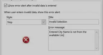
Question

How do you round to 2 decimal places in Excel?

wikiHow Staff Editor
Staff Answer
This answer was written by one of our trained team of researchers who validated it for accuracy and comprehensiveness.

wikiHow Staff Editor

Staff Answer

Go to the “Math & Trig” menu in the “Formulas” tab. Select “ROUND” from the drop-down menu. In the “Number” field, enter the number you want to the round or the ID of the cell containing the number. In the “Num_Digits” field, enter the positive integer “2” to indicate that you want 2 digits to appear after the decimal point.
Question

How do you round to the nearest whole number in Excel?

wikiHow Staff Editor
Staff Answer
This answer was written by one of our trained team of researchers who validated it for accuracy and comprehensiveness.

wikiHow Staff Editor

Staff Answer

When you use the “ROUND” function, enter a -1 in the “Num_Digits” field. This indicates that you want the rounding to happen just to the left of the decimal point, so you will round to a whole number instead of a decimal.
Question

How do you show 2 decimal places in Excel without rounding?

wikiHow Staff Editor
Staff Answer
This answer was written by one of our trained team of researchers who validated it for accuracy and comprehensiveness.

wikiHow Staff Editor

Staff Answer

To do this, you can use the TRUNC (“Truncate”) function. Write the formula =TRUNK, followed by 2 numbers in parentheses. The first is the number you want to truncate, the second is the decimal place you’d like to display. So, for instance, =TRUNC(27.3476,2) would give you 27.34, with no rounding.